Modeling Symmetries

Chaitanya K. Joshi's excellent blog post on his PhD work inspired me to write down some thoughts on symmetries and invariances in neural network models—particularly in the context of molecular data. Discussions around removing architectural biases can lean a little absolutist ("Bitter Lesson, GPUs go brrr!"), whereas the reality is more nuanced. I am actually not so opposed to the idea of encoding physical priors, but I am interested in when such symmetries should be embedded directly into the model architecture, and when they might be better handled implicitly: through data augmentation, regularization or inference-time tricks.

This post represents some of my current thinking on the topic, through the lens of two modeling domains in which the approaches to encoding symmetries are very different: neural network potentials and diffusion models.

Symmetries and Invariances

When modeling image data, there are many desirable invariances one can imagine (translation being the predominant one baked into the most common image model architecture, CNNs). Some of these invariances have questionable utility in practice, or do not match the statistics of a natural data distribution. Rotations of images fits this mold well - in theory, a classifier's ability to accurately predict an image attribute should not have too much to do with it's orientation. But requiring this invariance property removes a lot of information about the spatial distribution of colours and objects in images (skies are typically blue, and typically at the top of an image). If a model learns this bias from the data, is it incorrect?

How are symmetries different in molecular data?

When modeling molecular structures, we often have a larger number of possible symmetries to handle/respect than in a domain such as images, because they do not have an intrinsically informative orientation or scale. The most common symmetries we want to model are:

Permutation Symmetries - When we change ordering of atoms in a system, we want our model to produce the same result.
Rotation Symmetries - If we rotate our system, we want scalar values to be invariant and predicted forces to change with the same rotation
Translation Symmetries - Translating our system in absolute cartesian space does not affect our model.
Invariance with respect to a group action (e.g symmetry groups in materials)
Conservation of energy (this is a special case, because it is a symmetry of the dynamics of the system, not the configuration space)

Encoding symmetries in model architectures

Some of these symmetries are easier than others to encode into a model architecture by construction. For example, making a model translationally invariant requires that the model inputs contain only relative coordinates with respect to other atoms in the system. Permutation symmetries also fit well with the types of models that are commonly applied to molecular data (Graph Neural Networks and Transformers), which are easily made permutation invariant by construction.

Even symmetries which we believe are easy to encode in to a model architecture result in models with a bias toward certain models. For example, models which use relative coordinates between atoms are often biased toward edge heavy GNN models which use a lot of their parameters for processing edge representations, where the way to encode a finer grained representation of distance is to add more edges. This is particularly the case for models which encode edge distances in a PBC aware way, i.e the distance between two atoms is the minimum distance over a set of periodic images. Some more recent generative models of molecules disregard this architectural bias entirely by encoding atom positions as node features and either using a relative coordinate system with respect to a given basis, or by using data augmentation (e.g random translation) to make the model invariant to the choice of origin.

Sometimes encoding these symmetries is a concrete negative because of the way a model operates. For example, in a diffusion model of 3d coordinates, it can actually be easier to learn permutation symmetry through explicit encoding and augmentation. The reason for this is that during a diffusion process, you may have many atoms of the same type, which can diffuse to any of a given set of positions. A diffusion model of atoms has to learn to coordinate these atoms to form the correct structure, and learning to do this without an explicit atom index is difficult. Incidentally, this is the approach taken in All Atom Transformers, one of the first all atom generative models of molecules.

Although all of these symmetries are important, the rest of this post will focus on just two: equivariance with respect to rotations and conservation of energy. These two properties require the most careful consideration, and are the most difficult/expensive to encode into a model architecture. They are also distinct in an interesting way - equivariance is easy to learn from data, but conservation of energy is not.

Why is equivariance important for forcefields?

In the context of molecular forcefields, equivariance with respect to rotations is important because the physical properties we're modeling should not depend on our choice of coordinate system. A forcefield model predicts both scalar quantities (like total energy) and vector quantities (like atomic forces), and these should transform appropriately under rotations.

Equivariance with respect to rotations means that when we apply a rotation $R$ to our input coordinates, the model's outputs transform in a predictable way. For scalar quantities like energy, we want rotational invariance:

$E(R \cdot \mathbf{r}) = E(\mathbf{r})$

For vector quantities like forces, we want equivariance - the predicted forces should rotate by the same rotation applied to the input:

$\mathbf{F}(R \cdot \mathbf{r}) = R \cdot \mathbf{F}(\mathbf{r})$

where $\mathbf{r}$ represents the atomic coordinates and $R$ is a rotation matrix in $SO(3)$ . Methods to achive this have broadly fallen into 3 categories:

Equivariant Layers (Exact) - Layers which are designed to be equivariant to a given group action
Model Averaging (Approximate) - Average the model predictions over a set of rotations
Data Augmentation/Regularization (Approximate) - Apply a rotation to the input data, or regularize the model to learn an equivariant representation

Equigrad - continuous regularization for rotational equivariance

It is also possible to encourage a model to learn equivariant representations in a continuous manner using regularization. Equigrad, a method that we proposed in our Orb V3 paper, is one method for this.

Conceptually, we compute a gradient of the predicted energy $E$ with respect to an identity rotation matrix $\mathbf{R}$ that is inserted into the computational graph at the input. A nice way to achieve this is by first expressing an identity rotation $\mathbf{R}$ as the matrix exponential of a skew-symmetric null matrix, and then computing the gradient of $E$ with respect to that null matrix:

$\mathbf{R} = e^{\mathbf{G} - \mathbf{G}^T} \quad \text{and} \quad \Delta_{\text{rot}} = \frac{\partial E(\mathbf{r}^T \mathbf{R}, \mathbf{h} \mathbf{R})}{\partial \mathbf{G}}\bigg|_{\mathbf{G} = \mathbf{0}}$

where $\mathbf{r}$ are atomic positions and $\mathbf{h}$ is the cell matrix. This is quite a natural operation in the course of training a conservative forcefield model with rotations as a data augmentation, as we are already computing gradients of the energy with respect to the atomic positions, and already applying a rotation to the input. In practice this looks like:

def compute_rotation_gradient(energy, positions, rotation_matrix):
    # Compute the gradient of the energy with respect to the rotation matrix
    forces, rotation_gradient = torch.autograd.grad(
        energy, 
        grad_outputs=torch.ones_like(energy),
        inputs=[positions, rotation_matrix], 
        create_graph=True
    )
    return forces, rotation_gradient
 
def train_step(batch):
    positions, cell, target_energy, target_forces = batch
    # Compute the rotation matrix
    rotation_matrix = e3nn.nn.SO3.random()
    positions_rotated = positions @ rotation_matrix
    pred_energy, pred_forces = conservative_forcefield(
        positions_rotated, rotation_matrix
        )
    loss = (
        F.mse_loss(pred_forces, target_forces) + 
        F.mse_loss(pred_energy, target_energy) + 
        0.0001 * rotation_gradient.norm()
    )
    loss.backward()

Invariant models satisfy $\Delta_{\text{rot}} = \mathbf{0}$ by definition, because the predicted energy does not depend on the global orientation of the input coordinates and cell vectors. For non-invariant models trained with data augmentation, $\|\Delta_{\text{rot}}\|$ is naturally small but nonzero, and quantifies the hypothetical change in energy if a rotation were to be applied at the input. This is an interesting metric to track for a model, but we also use it as a regularizer to encourage the model to learn an equivariant representation. In practice, this works quite well and we see that models trained with this regularizer do learn a more equivariant representation.

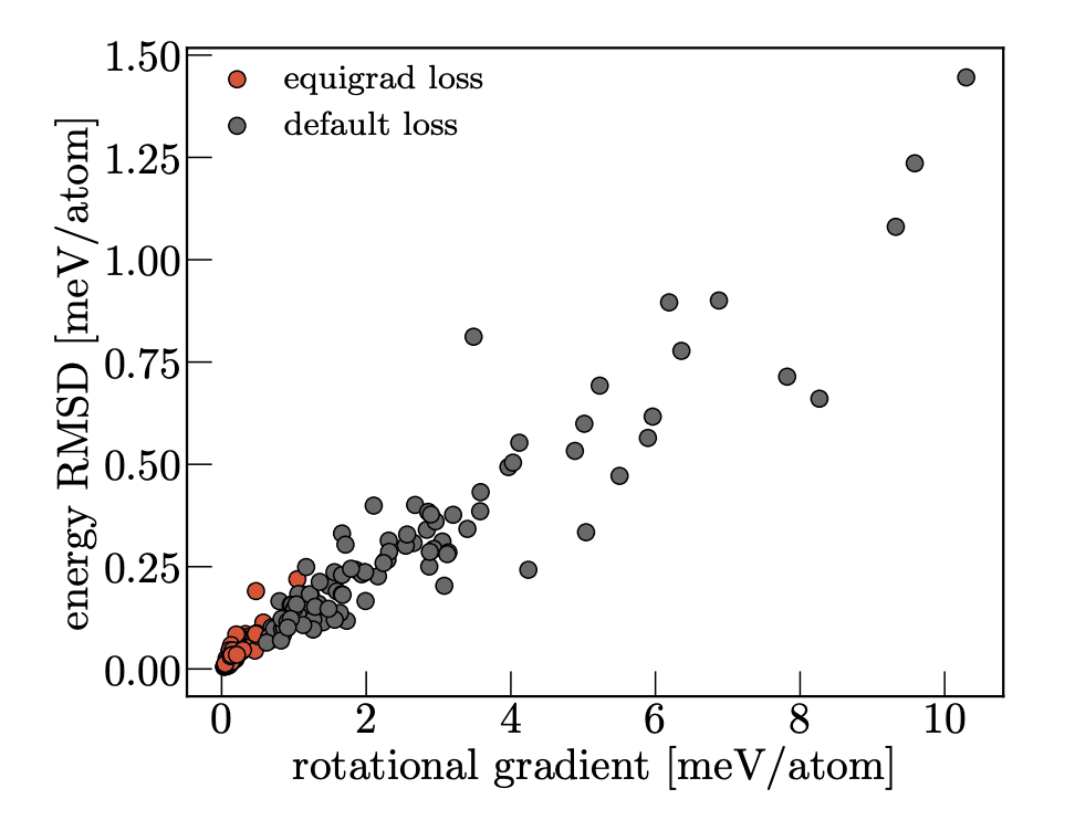
Equigrad is quite a "cute" method for making a model approximately equivariant to a group action, because it is a continuous regularization which can be applied to any model. It does have a few drawbacks - it is only applicable to conservative forcefields (as you need the gradient of the energy with respect to the rotation matrix), and it is quite a strong regularizer, which can make setting the appropriate scaling factor tricky in practice.

Model averaging is another common method for achieving approximate equivariance. Probing the effects of broken symmetries in machine learning explores the extent to which this affects measurement of observables in simulations which use non-equivariant models, and includes a discussion of model averaging as a method for achieving approximate equivariance.

A further argument for approximate equivariance is that it allows for more flexible models when the data distribution has broken or approximate symmetries (e.g. local disorder, noisy experimental data, crystal phase transitions). In order to model this, there is work on adapting equivariant models to model the highest level of symmetry consistent with the data (e.g Relaxed EGNNs, Imperfectly Symmetric Dynamics). To me, these papers are academically interesting, but in practice seems like a problem in search of a solution; we have methods for approximate equivariance which allow smooth interpolation between the two extremes of exact equivariance and no equivariance (data augmentation, model averaging and regularization) without having to make the model architecture more complex.

Scaling laws and equivariance

Two recent papers have claimed to show that equivariant models actually scale better than non-equivariant models. Does equivariance matter at scale? and Probing Equivariance and Symmetry Breaking in Convolutional Networks. These papers make some valuable contributions in terms of understanding the scaling properties of equivariant models, but I continue to be a bit skeptical of the claims made in these papers, for two reasons:

It is important to measure wallclock time, not just flops. Unconstrained models typically have a larger number of flops, but this is not representative of how fast they can actually run. Of course, this does depend on hardware/implementation, but sometimes this is an intrinsic property of the model architecture. Transformers are very fast on GPUs because of their highly optimized implementation, but algorithmically they were designed for exactly this purpose.
They typically use small molecular datasets like QM9 (both in terms of number of atoms, and number of systems). This is not representative of most molecular datasets today, and is not representative of the scale of systems we want to model.

One common motivation for using equivariant models is their data efficiency in the small data regime, and commonly it is demonstrated that this gap can be narrowed using data augmentation. This is disregarded as an unsatisfactory solution in these papers because it would increase training time. However, in my experience non-equivariant models can be 1-2 orders of magnitude faster and more memory efficient, erasing this gap in practice.

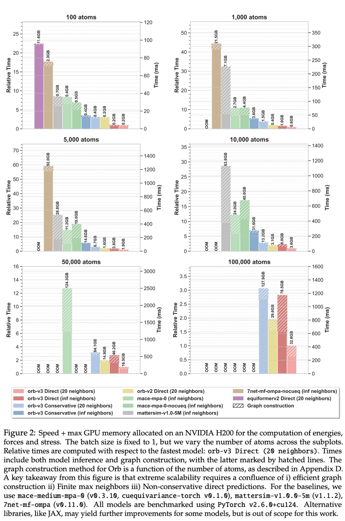
Our speed benchmark from the Orb V3 paper is below. This shows a practical comparison of the speed of a variety of models on a range of system sizes. Looking at scaling with respect to the number of atoms up to the 100k range may not be representative of most molecular datasets today, but it is important not to limit the scale of our ambition - if we want to model mesoscale systems like proteins, it is critically important that build models which can scale to this range.

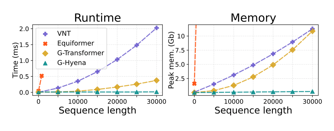
I am actually quite excited about newer equivariant architectures which address some of the scalability issues of previous approaches (particularly with respect to the number of atoms in a system). Geometric Hyena Networks (a spotlight at ICML this year) is one such example.

Conservative Vector fields

Conservation of energy requires that the forces produced by the model are the gradient of a potential energy function. A vector field $\mathbf{F}$ is conservative if there exists a scalar potential function $U$ such that:

$\mathbf{F} = -\nabla U$

This implies that the curl of the force field is zero: $\nabla \times \mathbf{F} = 0$ , and that the work done by the force field is path-independent.

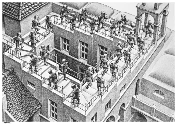
This most intuitive explanation of this property is the analogy of Escher's staircase. On Escher's staircase, it is possible to traverse between two points on the stairs in two ways - either by going up, or by going down. If we were to consider the energy landscape of the staircase, we would see that there are two different paths between the same two points, and that the energy of the system is different on each path. A vector field being conservative means that the energy requires to move between two points is the same no matter which path is taken, meaning that Escher's staircase is unphysical - because walking upstairs to get to a point would require more energy than walking downstairs.

The way the implementation of a conservative vector field manifests itself in a neural network based forcefield model is that the forces are defined as the gradient of the energy with respect to the atomic coordinates, and the entire model is trained with double backprop:

 
def conservative_forcefield(positions, atomic_numbers):
    
    energy = energy_network(positions, atomic_numbers)
    # Compute forces as negative gradient of energy
    forces = -torch.autograd.grad(
        outputs=energy,
        inputs=positions,
        grad_outputs=torch.ones_like(energy),
    )[0]
    return energy, forces
 
def train_step(batch):
    positions, atomic_numbers, target_energy, target_forces = batch
    pred_energy, pred_forces = conservative_forcefield(
        positions, atomic_numbers
        )
    # Compute losses
    energy_loss = F.mse_loss(pred_energy, target_energy)
    force_loss = F.mse_loss(pred_forces, target_forces)
    
    total_loss = energy_loss + force_loss
    # Second backprop
    total_loss.backward()

Orb V1/2 were trained as direct models, and as such we observed that they did not conserve energy, particularly under NPT MD conditions. Orb V3 contained our first set of models that were conservative. Hopefully this emphasises that I am not fundamentally against baking in important properties of a system into a model - we could not find a good way to approximate energy conservation in a forcefield effectively, so we built new models with this property baked in.

Conservative models are very interesting! In particular, they are common in the context of forcefields, but they also have an analogous interpretation in the machine learning literature: Energy Based Models (EBMs). The next section explores this connection, and in particular looks at diffusion models as a very successful class of models which avoid encoding this conservation property into a model architecture.

Forcefields are secretly unnormalized Energy Based Models

Forcefields can be viewed as unnormalized Energy Based Models (EBMs) trained with direct supervision. Forcefields define a deterministic energy function $E(r)$ over atomic coordinates $r$ , and forces are given by: $F = -\nabla_r E(r)$ . This is used extensively in MD by defining a Boltzmann distribution over the atomic coordinates, which is equivalent to the distribution of the system under the forcefield. If you interpret $p(r) \propto e^{-E(r)/kT}$ as the probability of a configuration $r$ , then the forcefield is the gradient of the log of this probability (up to a constant factor at a given temperature).

The main difference is the method of training - in other areas of machine learning, it is very unusual to have access to energies and gradients of the potential function you are trying to model. A large swathe of ML literature is concerned with how to train EBMs (e.g Contrastive Divergence, Maximum Likelihood with MCMC, NCE), or approximate models of the score function (Score Matching, Denoising Diffusion Implicit Models) which do not require a tractable normalising constant.

Score matching and Diffusion as Energy Based Model Approximations

One particularly interesting approximation of EBMs are diffusion models. These models are trained to approximate the score function of the data distribution, where the score matching objective is specifically designed to avoid the need to explicitly define or compute an energy function.

The score function is defined as the gradient of the log probability density:

$s(x) = \nabla_x \log p(x)$

In the context of EBMs, if we have an energy function $E(x)$ and define $p(x) = \frac{1}{Z} e^{-E(x)}$ where $Z$ is the partition function, then:

$s(x) = \nabla_x \log p(x) = \nabla_x \log \left(\frac{1}{Z} e^{-E(x)}\right) = -\nabla_x E(x)$

The score matching objective avoids computing the intractable partition function $Z$ by matching the score directly. The denoising score matching objective used in diffusion models is:

$\mathcal{L} = \mathbb{E}_{x_0 \sim p_{data}, \epsilon \sim \mathcal{N}(0, I), t} \left[ \left\| s_\theta(x_t, t) + \frac{\epsilon}{\sigma_t} \right\|^2 \right]$

where $x_t = x_0 + \sigma_t \epsilon$ is the noised data at time $t$ , and $s_\theta(x_t, t)$ is the neural network approximating the score function.

Conservative Diffusion models

It is possible to define a model of the score function in a similar way to the adaptations one makes for a conservative forcefield, namely defining an energy function and defining your score as the gradient of the log of this energy function, even when the energy function is not explicitly defined for domains such as images:

$s_\theta(x) = -\nabla_x E_\theta(x)$

where $E_\theta(x)$ is a neural network parameterizing (a synthetic, unknown) energy function, and the score is computed via automatic differentiation.

image = torch.randn(1, 3, 10, 10)
noise = torch.randn_like(image) * 0.1
noised = image + noise
model = torch.nn.Sequential(
    torch.nn.Conv2d(3, 16, 3),
    torch.nn.ReLU(),
    torch.nn.Conv2d(16, 1, 3)
)
 
energy = model(noised)
score = torch.autograd.grad(energy, noised)
loss = F.mse_loss(score, noise)
loss.backward()

This idea has been explored in Reduce, Reuse, Recycle: Compositional Generation with Energy-Based Diffusion Models and MCMC and discussed in Should EBMs model the energy or the score?. The second paper, (a very clear exposition of the relationship between EBMs and diffusion models) does include the following quote: "in personal communication multiple researchers in this area indicated that they did not obtain good results following this approach.". This is likely because defining a model in this way requires a 2x increase in memory use and training time, due to the two gradient computations.

Why Conservative NNPs but not Conservative Diffusion models?

Applications of diffusion models, regardless of domain, should desire all of the properties that a conservative vector field brings - after all, sampling from a diffusion model also uses various forms of annealed Langevin dynamics, which is only guaranteed to draw samples from the true data distribution if the forcefield is conservative. It would also be beneficial for a diffusion model to be able to compare relative energies of different samples. Knowing the energy function would also enable the use of more advanced MCMC techniques when sampling, such as Hamiltonian Monte Carlo. Despite this, diffusion models are the best performing generative models by some margin for a wide range of domains.

It is possible that defining conservative models of the score function has been under-explored. However, given the massive popularity of diffusion models (and the quote from multiple researchers in the paper), I think it is likely that the performance tradeoff required to make diffusion models produce a conservative vector field is either 1) not worth the added complexity, or 2) does not scale to the size of the top performing diffusion models. This is a good example of scalability being a major factor in the design of neural network models - we sacrifice some properties of the model in order to make it more scalable.

Takeaway

All of this discussion to say - we desire conservative, equivariant forcefield models because the applications we use them in make heavy use of the ability to produce physical dynamics, determine a sample's energy under a model, and by extension the ability to compare relative energies of different samples. However, there is room for caution in this approach, because empirically, the best models for density estimation in many other modalities skirt around this explicit modeling.

Direct forcefield models are an example of the trade-off between energy conservation and equivariance vs model scalability. It is not that ML researchers are unaware of the importance of energy conservation, or equivariance, but that we have seen in other contexts that achieving these properties by encoding them into a model architecture is not always the best choice, and that sometimes these properties can be accessed in a different way. For example, newer, continuous parameterizations of diffusion models as ODEs can access exact log likelihoods for individual samples via Hutchinson's estimator, allowing comparison of relative samples, or averaging over rotations of a system at runtime allows an approximation of equivariance up to an arbitrary precision. These types of indirect approaches often results in models which can get the best of both worlds up to some approximation, so it's important to view these seemingly "brute force" approaches with the idea that they may have something to add to the conversation. I'm excited about developing the right tools for representing the constraints at hand, whilst being open to the idea that approximate symmetry might be good enough, or even better, when deployed at scale.